Overview
Abstract
The Environment system contains and controls everything external to the patient and equipment (e.g. Anesthesia Machine Methodology). It sets the ambient boundary conditions for both fluid and thermal systems. The Environment system provides a means to add airborne substance values, and calculates the heat transfer due to convection (natural and forced), radiation, and evaporation.
Introduction
The Environment system defines the ambient conditions for the body. The Environment system controls everything from the phase of the environmental fluid (i.e. gas when is a room or liquid when submerged in water) to the volume fractions of constituent gases in the environmental fluid when that fluid is a gas. The Environment system also computes heat exchange between the body and the environment as well as and substance delivery to the body-environment interfaces.
System Design
Background and Scope
The many physiological functions within the human body depend heavily on the conditions of the environment within which the body is located. Thus, the Environment system is required to determine patient boundary conditions to enable a generic, extensible approach to modeling physiology within the body. Though the Common Data Model and Software Framework (CDM), the Environment system interacts with and informs other systems, particularly the Respiratory, Cardiovascular, and Energy systems, and the Environment system was developed to include hooks for future integration into various applications such as games and sensor systems.
Requirements
The Environment system is used to meet the following requirements:
- Meteorological effects
- Surrounding atmospheric gas properties, including pulmonary agent exposure
- Altitude effects
- Heat transfer into and out of the skin and lungs
- Clothing resistances
- Ambient temperature changes
- Ambient humidity changes
- Multiple surrounding fluid types (i.e. submerged in water vs. air)
- Air velocity effects on convection
- Solar and surrounding material (i.e. walls) considerations
- Active heating and cooling
Previous Research
One of the most comprehensive analysis of human interaction with typical thermal environments is contained within the American Society of Heating, Refrigerating, and Air-Conditioning Engineers (ASHRAE) Handbook - specifically the Thermal Comfort chapter [153]. The International Organization for Standardization (ISO) standard 7730:2005: Ergonomics of the Thermal Environment contains additional data and analyses [171]. Both of these publications are focused on occupant thermal comfort for indoor environment planning and thus make assumptions that are not valid for some of the extreme environments required by the engine. Data and analyses from these publications were heavily leveraged during development of the environment system. Other existing research includes the high-level heat transfer analysis focused on medical and biological applications reported in Ref. [321], as well as experimental and computational explorations of thermoregulation [224] [255] [76] [117].
Approach
The Environment system was designed with as few assumptions and parameter bounds as possible to allow simulations of both standard and extreme environments. The system is dynamic. By leveraging the Common Data Model and Software Framework and the generic circuit and convective transport solvers, the engine will react differently to varying initial environments and to changes in the environment during simulation. Environment parameters can be changed through specifying a separate environment file, or by manually updating the parameters through the environment state change action (for more details see the SDK). Table 1 shows these inputs, which set the substance, fluid, and thermal properties external to the patient.
| Parameter | Use | Unit Type |
|---|---|---|
| Air Density | Thermal | MassPerVolume |
| Air Velocity | Thermal | LengthPerTime |
| Ambient Temperature | Thermal | Temperature |
| Atmospheric Pressure | Fluid | Pressure |
| Clothing Resistance | Thermal | HeatResistanceArea |
| Emissivity | Thermal | Fraction |
| Mean Radiant Temperature | Thermal | Temperature |
| Relative Humidity | Thermal | Fraction |
| Respiration Ambient Temperature | Thermal | Temperature |
| Ambient Substance | Substance | Fraction |
The Thermal Application action is handled by the Environment system and has the following options (with unit type):
- Active Heating
- Heating Power (Power)
- Heated Surface Area Fraction (Fraction)
- Heated Surface Area (Area)
- Active Cooling
- Cooling Power (Power)
- Cooled Surface Area Fraction (Fraction)
- Cooled Surface Area (Area)
- Applied Temperature
- Applied Temperature (Temperature)
- Applied Surface Area Fraction (Fraction)
- Applied Surface Area (Area)
Substance Environment
Ambient substance volume fractions can be modified through the Environment system. The environmental fraction of typical atmospheric gases (e.g. O2, CO2, N2, etc.) and concentrations of airborne agents in suspension (i.e. aerosols) can be set and/or dynamically adjusted. The gases and aerosols enter the Respiratory System with the generic convective Substance Transport Methodology.
Fluid Environment
Many meteorologic parameters such as ambient temperature, wind speed, atmospheric pressure, and humidity are set and used by the Environment system. The atmospheric pressure is set directly on the Respiratory and Anesthesia Machine reference (ambient) node values, which automatically propagates effects throughout. The other thermal values are used to determine the Environment circuit element values described in more detail below.
Thermal Environment
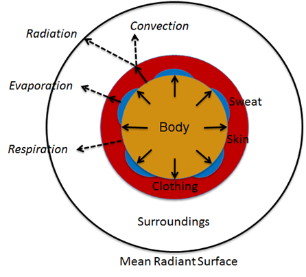
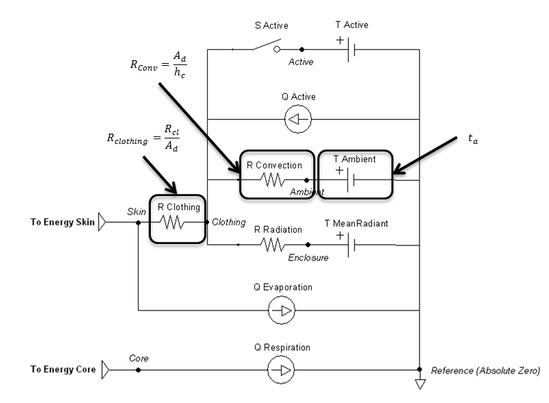
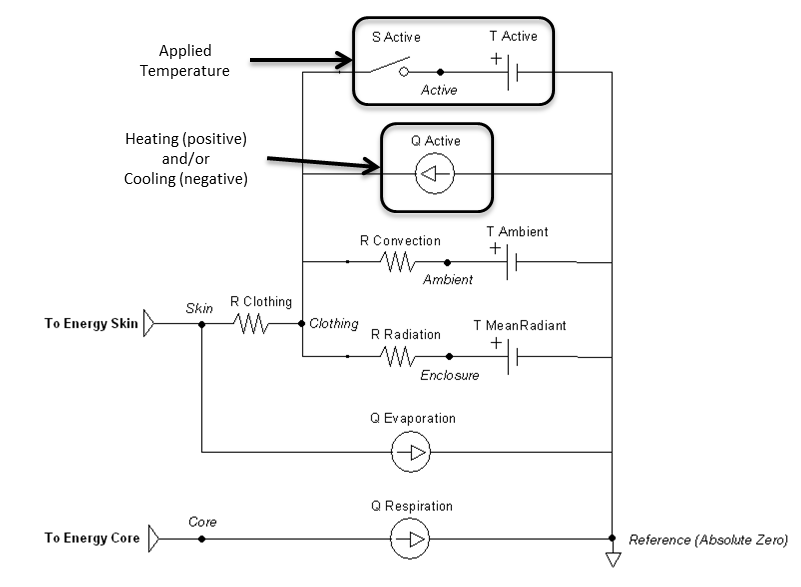
The remaining parameters are used for setting and manipulating the surrounding thermal environment. A simplified one-dimensional representation of the thermodynamic process solved by the Environment system is shown in Figure 1 [153] . The Environment circuit connects directly to the Energy system circuit to balance with metabolic rate and body heat storage.
Data Flow
Initialize
During resting stabilization, the patient reaches a homeostatic value using the standard environment. Following that steady-state starting point, the user has the option to modify any environment values as a condition. The simulation will not start running until a new steady-state is achieved using these new parameters.
Preprocess
Preprocess uses feedback to calculate thermal properties and circuit element values for the next engine state. The Preprocess methods are described in more detail in the next section.
Process
The generic circuit methodology developed for the engine is used to solve for the pressure, flow, and volume at each node or path. For more details, see the Circuit Methodology.
Post Process
The Post Process step moves everything calculated in Process from the next time step calculation to the current time step calculation. This allows all other systems access to the information when completing their Preprocess analysis for the next time step.
Features and Capabilities
Definitions
Acronyms and a nomenclature table are available in the appendix.
Circuit
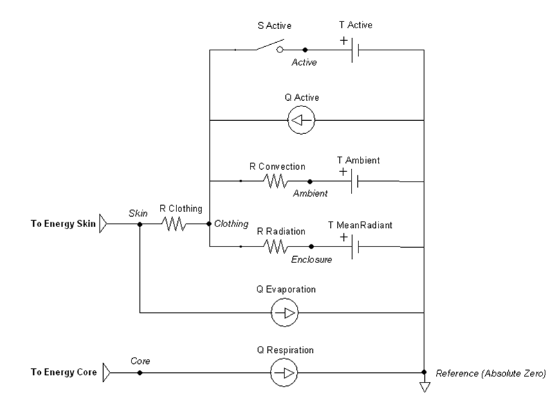
The one-dimensional model shown in Figure 1 is further simplified to a zero-dimensional model (Figure 3) by averaging the thermal effects over the entire patient. The Environment system uses the generic circuit solver in the same way as fluid systems (Circuit Methodology).
The Ambient node contains both thermal properties (temperature), fluid properties (pressure), and substance properties (volume fraction, aerosol concentration). It is assigned as the Respiratory and Anesthesia Machine circuit’s reference node, and therefore, interacts with them directly. Any changes to the Ambient node properties automatically propagates through the other systems.
The clothing thermal insulation/resistance in this model is an average lumped value over the entire patient's body. Because clothing insulation cannot be measured for most routine engineering application, tables of measure values for various ensembles can be used as in Table 2 [153]. When a premeasured ensemble cannot be found to match, estimated ensemble insulation can be determined via a summation of the individual garmets as in Table 3 [153]. An important note is that the clothing resistance remains constant once set, and does not automatically take into account sweat saturation or changes due to submersion. These effects could be accounted for by external determination of a new thermal resistance value and set using the environment change action.
| Ensemble Description | Icl (clo) |
|---|---|
| Walking shorts, short-sleeved shirt | 0.36 |
| Trousers, short-sleeved shirt | 0.57 |
| Trousers, long-sleeved shirt | 0.61 |
| Same as above, plus suit jacket | 0.96 |
| Same as above, plus vest and T-shirt | 0.96 |
| Trousers, long-sleeved shirt, long-sleeved sweater, T-shirt | 1.01 |
| Same as above, plus suit jacket and long underwear bottoms | 1.30 |
| Sweat pants, sweat shirt | 0.74 |
| Long-sleeved pajama top, long pajama trousers, short 3/4 sleeved robe, slippers (no socks) | 0.96 |
| Knee-length skirt, short-sleeved shirt, panty hose, sandals | 0.54 |
| Knee-length skirt, long-sleeved shirt, full slip, panty hose | 0.67 |
| Knee-length skirt, long-sleeved shirt, half slip, panty hose, long-sleeved sweater | 1.10 |
| Knee-length skirt, long-sleeved shirt, half slip, panty hose, suit jacket | 1.04 |
| Ankle-length skirt, long-sleeved shirt, suit jacket, panty hose | 1.10 |
| Long-sleeved coveralls, T-shirt | 0.72 |
| Overalls, long-sleeved shirt, T-shirt | 0.89 |
| Insulated coveralls, long-sleeved thermal underwear, long underwear bottoms | 1.37 |
| Garment Description | Icl (clo) | Garment Description | Icl (clo) |
|---|---|---|---|
| Underwear | Dress and Skirts | ||
| Bra | 0.01 | Skirt (thin) | 0.14 |
| Panties | 0.03 | Skirt (thick) | 0.23 |
| Men's briefs | 0.04 | Sleeveless, scoop neck (thin) | 0.23 |
| T-shirt | 0.08 | Sleeveless, scoop neck (thick), i.e., jumper | 0.27 |
| Half-slip | 0.14 | Short-sleeve shirtdress (thin) | 0.29 |
| Long underwear bottoms | 0.15 | Long-sleeve shirtdress (thin) | 0.33 |
| Full slip | 0.16 | Long-sleeve shirtdress (thick) | 0.47 |
| Long underwear top | 0.20 | ||
| Footwear | Sweaters | ||
| Ankle-length athletic socks | 0.02 | Sleeveless vest (thin) | 0.13 |
| Pantyhose/stockings | 0.02 | Sleeveless vest (thick) | 0.22 |
| Sandals/thongs | 0.02 | Long-sleeve (thin) | 0.25 |
| Shoes | 0.02 | Long-sleeve (thick) | 0.36 |
| Slippers (quilted, pile lined) | 0.03 | ||
| Calf-length socks | 0.03 | Suit Jackets and Vests (lined) | |
| Knee socks (thick) | 0.06 | Sleeveless vest (thin) | 0.10 |
| Boots | 0.10 | Sleeveless vest (thick) | 0.17 |
| Shirts and Blouses | Single-breasted (thin) | 0.36 | |
| Sleeveless/scoop-neck blouse | 0.12 | Single-breasted (thick) | 0.44 |
| Short-sleeve knit sport shirt | 0.17 | Double-breasted (thin) | 0.42 |
| Short-sleeve dress shirt | 0.19 | Double-breasted (thick) | 0.48 |
| Long-sleeve dress shirt | 0.25 | ||
| Long-sleeve flannel shirt | 0.34 | Sleepwear and Robes | |
| Long-sleeve sweatshirt | 0.34 | Sleeveless short gown (thin) | 0.18 |
| Trousers and Coveralls | Sleeveless long gown (thin) | 0.20 | |
| Short shorts | 0.06 | Short-sleeve hospital gown | 0.31 |
| Walking shorts | 0.08 | Short-sleeve short robe (thin) | 0.34 |
| Straight trousers (thin) | 0.15 | Short-sleeve pajamas (thin) | 0.42 |
| Straight trousers (thick) | 0.24 | Long-sleeve long gown (thick) | 0.46 |
| Sweatpants | 0.28 | Long-sleeve short wrap robe (thick) | 0.48 |
| Overalls | 0.30 | Long-sleeve pajamas (thick) | 0.57 |
| Coveralls | 0.49 | Long-sleeve long wrap robe (thick) | 0.69 |
Aerosol
An aerosol is a colloidal suspension of either solid or liquid droplet particles suspended in a gas (typically the surrounding air). Real aerosols can be monodispersed but are more often polydispersed, having a range of particle diameters. Particle deposition and retention in the lung depends on a number of, factors including particle aerodynamic diameter [55] [245]. Other deposition factors, including inhalation flow rate and tidal volume [193], are accounted for by the breathing patterns simulated by the engine. In order to avoid the computational cost of tracking millions of individual particles or many groups of particles in a distribution throughout the respiratory tract and into the body, aerosols are modeled as a single concentration in the environment. The location of deposition and the deposition efficiency at each location is determined by first computing a particle-size-independent deposition efficiency for each compartment from a defined size-distribution histogram. The size-independent deposition efficiencies are computed from the deposition fractions which are determined for each compartment from the particle diameter using the equations fit by Hinds to the ICRP66 simulation results [165], as described by [301]. The deposition fraction equations from [301] are plotted in Fig. 4, and example mean depositions fractions for a particular histogram are shown. For the model implementation it is assumed that all particles are spherical, thus diameter is the aerodynamic diameter.
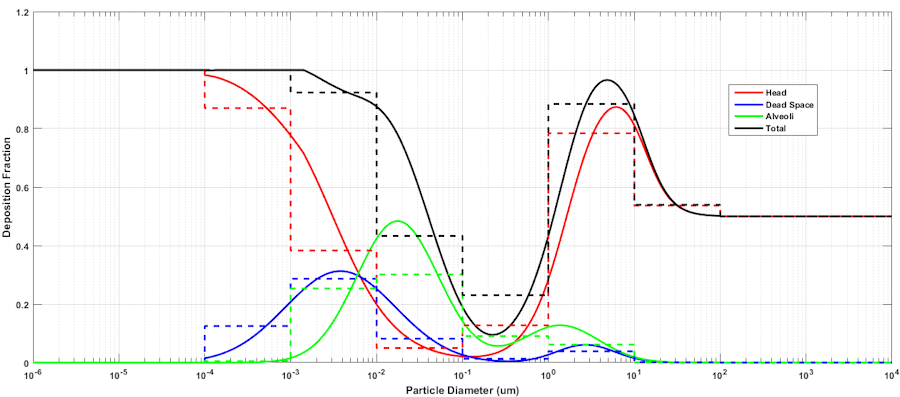
The size-independent deposition efficiencies are computed from the deposition fractions using Equation 31.
![\[\mathrm{K_B=}\frac{\left( b_1f_1 + \cdots + b_nf_n \right)}{\left( \left( 1-a_1 \right)f_1 + \cdots + \left(1-a_n \right)f_n \right)} \]](form_51.png)
Here *KB* is the size independent deposition efficiency coefficient for compartment B, *bi* is the fraction of total particles of size i entering the body that deposit in compartment B, and *fi* is the fraction of total particles in the environment that are of size i. Likewise, *ai* is the fraction of total particles of size i entering the body that deposit in compartment A. This equation is derived by first considering a polydispersed aerosol with particles divided by size into n number of bins. The total mass of particles in an aliquot of to-be-inhaled air prior to inhalation is equal to the sum of the masses of the particles in each bin, as described by Equation 2.
![\[m_t = \Sigma_{i=1}^{n}m_i \]](form_52.png)
The mass of the particles in each bin must be defined by a fraction specified in a histogram. The size of the histogram is arbitrary. The only requirement is that a histogram is supplied rather than a density function. Equation 3 describes the mass of particle i within the aliquot of aerosol.
![\[m_i = f_im_t \]](form_53.png)
Likewise, the total mass of particles in compartment A is equal to the sum of the masses of the particles in each bin, and the same is true for compartments B, C, D, etc., described by Equation 4.
![\[m_{tA} = \Sigma_{i=1}^{n}m_{iA} \]](form_54.png)
The mass of particles in compartment B is also equal to the mass of the particles that did not deposit in the adjacent upstream compartment A.
![\[m_{iB} = \left(1-a_i \right)m_i \]](form_55.png)
Combining Equations 2-5 yields Equation 6.
![\[m_{iB} = \left( \left(1-a_1 \right)f_1 + \cdots + \left(1-a_n \right)f_n \right)m_t \]](form_56.png)
The total mass of particles that deposit in compartment B is some fraction of the total particles in compartment B, which is the sum of the amount deposited from each bin in compartment B.
![\[K_{B}m_{tB} = \left(b_1f_1 + \cdots + b_nf_n \right)m_t \]](form_57.png)
Rearranging Equation 7 and combining with Equation 6 yields Equation 1, the size-independent deposition efficiency coefficient for compartment B.
The mass deposited in each compartment is computed by multiplying the size-independent deposition efficiency coefficient by the mass in the compartment at each time step. Once an aerosol substance deposits in a respiratory compartment it stays in the respiratory compartment. In other words, coughing is not productive in the engine. The direct effect of a deposited substance depends on the mass deposited and the value of the inflammation coefficient that is defined in the substance file. The inflammation coefficient defines the amount of damage, by any mode, that the substance does to the respiratory tissue. Figure 5 visually describes the direct effects of an aerosol on the Respiratory system.
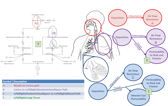
In addition to the direct effects, deposited aerosol substances can also have indirect effects. After liquid aerosol substances deposit they can diffuse into the surrounding tissue and then into the blood stream. If the liquid aerosol has pharmacodynamic properties defined, it's effects will be realized when it enters the blood and the plasma concentration becomes non-zero.
Currently, Albuterol and smoke particulate have histogram data and are modeled as polydisperse aerosols in the environment with the former being delivered via an inhaler and the latter being a concentration in the ambient environment. Smoke is modeled as a solid aerosol.
The solid smoke particulate in the engine is a model of the particulate generated through the combustion of organic material in a forest fire. We assume that the fire is well evolved in time to mitigate the bi-modal behavior seen during the initial ignition and smoldering [396]. This allows us to model the size distribution as a lognormal curve. The forest fire smoke particle size distribution histogram is given in table 4.
| Amount (fraction) | Diameter (microns) |
|---|---|
| 0.015 | 1.0e-4 - 1.0e-3 |
| 0.035 | 1.0e-3 - 1.0e-2 |
| 0.9 | 1.0e-2 - 1.0e-1 |
| 0.035 | 1.0e-1-1.0 |
| 0.015 | 1.0-1.0e1 |
| 0 | 1.0e1 - 1.0 e2 |
Figure 6 summarizes the fate and effects of liquid and smoke aerosols in the engine. 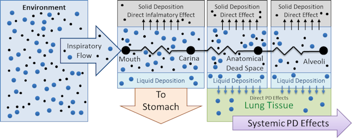
Carbon Monoxide
Carbon monoxide (CO) is a toxic gas that is odorless, colorless, and tasteless. Carbon monoxide binds to the ferrous-heme site of the hemoglobin molecule in the same way that oxygen does (it also cannot bind to the oxidized methemoglobin sites), thus the maximal oxygen capacity falls to the extent that CO is bound. The subunits of the hemoglobin molecule are collectively in a tense state (T) or a relaxed state (R). All four subunits are always in the same state. The hemoglobin molecule is in the tense state when less oxygen is bound and it has a lower affinity for oxygen in the T state. When enough oxygen is bound, all subunits snap into the R state whether or not they are bound to oxygen, and the hemoglobin molecule has ~150 times the affinity for oxygen. It is this snapping that creates the steep portion of the binding curve and allows for the reversible carriage of oxygen by the blood. Like oxygen, as carbon monoxide binds to hemoglobin it can push the molecule from the relaxed to the tensed state, thus increasing the affinity for oxygen and reducing the amount of oxygen released from the hemoglobin molecule when it enters the oxygen depleted systemic capillaries. Additionally, carbon monoxide binds competitively to hemoglobin. For every molecule of CO bound to a heme site, there is one less site for oxygen to bind. The net result of these two phenomena, but predominately due to the former, is that there is less oxygen delivery to the tissues when CO is present in the blood.
There are three components to the carbon monoxide model: transfer across the alveolar membrane, binding to hemoglobin, and the effects of binding on the oxygen binding curve. Obviously these three components are interrelated. As CO binds to hemoglobin in the pulmonary capillaries, less CO is dissolved in fluid and therefore the partial pressure gradient between the alveoli and the pulmonary capillary blood is higher, driving an increase in Fick's law diffusion resulting in more carbon monoxide in the blood. As more CO enters the blood, more binds to hemoglobin and the oxygen-hemoglobin saturation curve shifts to the left. The alveolar transfer of carbon monoxide is simulated by assuming that the membrane diffusivity of CO is similar to oxygen and then by leveraging the alveolar exchange model described in the Tissue Methodology report. Models for the binding of CO to hemoglobin and the effects on the oxygen saturation curve are discussed separately below.
Carbon Monoxide Binding
The distribution of carbon monoxide species (dissolved and bound to hemoglobin) in each vascular compartment is computed from the conservation of mass and the Haldane relationship described in [46]. Canservation of mass is described by Equation 8.
![\[T_{CO} = CO_{Hb} + k_{CO}P_{CO} \]](form_58.png)
where *TCO* is the total carbon monoxide in the blood, *COHb* is the carbon monoxide bound to hemoglobin, *PCO* is the partial pressure of carbon monoxide in the blood, and *kCO* is the Henry's Law solubility coefficient for carbon monoxide. Equation 9, the Haldane relationship, provides the second equation necessary to solve for the two unknown values. In Equation 9, *MH* is the Haldane affinity ratio for hemoglobin, *Pgas* is the partial pressure of the gas, and *GasHb* is the amount of gas bound to hemoglobin.
![\[M_H \frac{P_{CO}}{CO_{Hb}} = \frac{P_{O_2}}{O_{2_{Hb}}} \]](form_59.png)
The model is implemented by first totaling the carbon monoxide in a compartment post diffusion, then computing the partial pressure of carbon monoxide, and finally computing the carboxyhemoglobin in the compartment. After the target distribution is calculated, the hemoglobin species (unbound, oxyhemoglobin, carboxyhemoglobin, carbaminohemoglobin, and oxycarbaminohemoglobin) amounts are updated by assuming that unbound hemoglobin is consumed first followed by oxyhemoglobin then oxycarbaminohemoglobin and finally carbaminohemoglobin. If all hemoglobin is converted to carboxyhemoglobin before the necessary adjustment is made to conserve CO mass, then the remaining CO is distributed back to the dissolved species. This acts as an automatic negative feedback device to ensure that the perfusion contribution to the diffusing capacity is saturated when the hemoglobin becomes saturated. See the C++ code for more details.
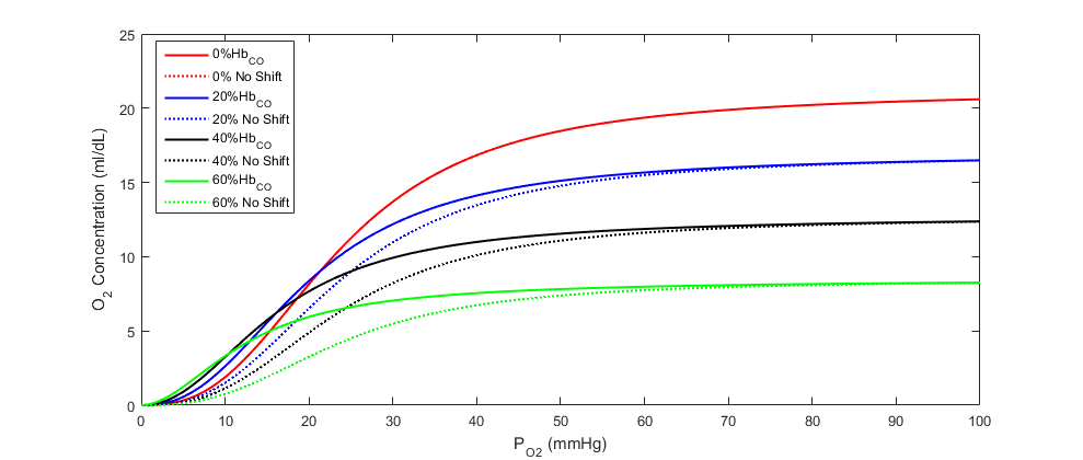
Carbon Monoxide Effects on Oxygen Saturation Curve
The oxygen saturation curve effects model implemented is adapted from the regression model described by bruce2003multicompartment. We have simplified the model by assuming a linear relationship between carboxyhemoglobin and both the Hill coefficient and the 50% saturation shaping parameter. We then applied the linear relationship to the Dash and Bassingthwaithe oxygen saturation model already implemented in the engine (see the Tissue Methodology). Equations 10 and 11 describe the adjustments made to the oxygen saturation curve in the presence of carboxyhemoglobin, and Figure 7 shows the shift in the curve at various carboxyhemoglobin concentrations. In the equations, η is the Hill coefficient, *SCO* is the fraction of carboxyhemoglobin to total hemoglobin (i.e. CO saturation), and *P50* is the standard partial pressure of oxygen at 50% oxygen saturation.
![\[\eta = 1.7 - 1.1 \cdot S_{CO} \]](form_60.png)
![\[P_{50} = 26.8 - 20 \cdot S_{CO} \]](form_61.png)
Dependencies
The Environment circuit is directly connected through the skin and core to the Energy system for full body thermoregulation. This boundary condition feedback in and out is automatically handled through the node and path interactions. It also shares an ambient node with the Respiratory and Anesthesia Machine systems.
The Environment system relies on inputs from several other systems. The sweat rate from the Energy system is needed to determine the amount of heat lost through convection and evaporation. The respiration rate from the respiratory system is needed to determine the amount of heat lost via the respiratory track.
Supplemental Values
Numerous patient and thermal properties are determined and set in the supplemental values method for later calculations.
Since the one dimensional model used for the Environment thermal circuit needs to be averaged over the patient’s skin surface area, an approximate value must be determined. The most widely used equation to determine body surface area without direct measurement is the Du Bois formula presented in Equation 12 [153] , where mass is in kg and height is in m.
![\[{A_d}{\rm{ = 0}}.{\rm{202}}{m^{{\rm{0}}.{\rm{425}}}}{l^{{\rm{0}}.{\rm{725}}}}\]](form_62.png)
Several properties of water are needed at varying temperatures to determine the heat transfer occurring between the skin/clothing/lungs and the air. Four of these are determined using the best fit of property tables or experimental data, as shown in Figure 8.
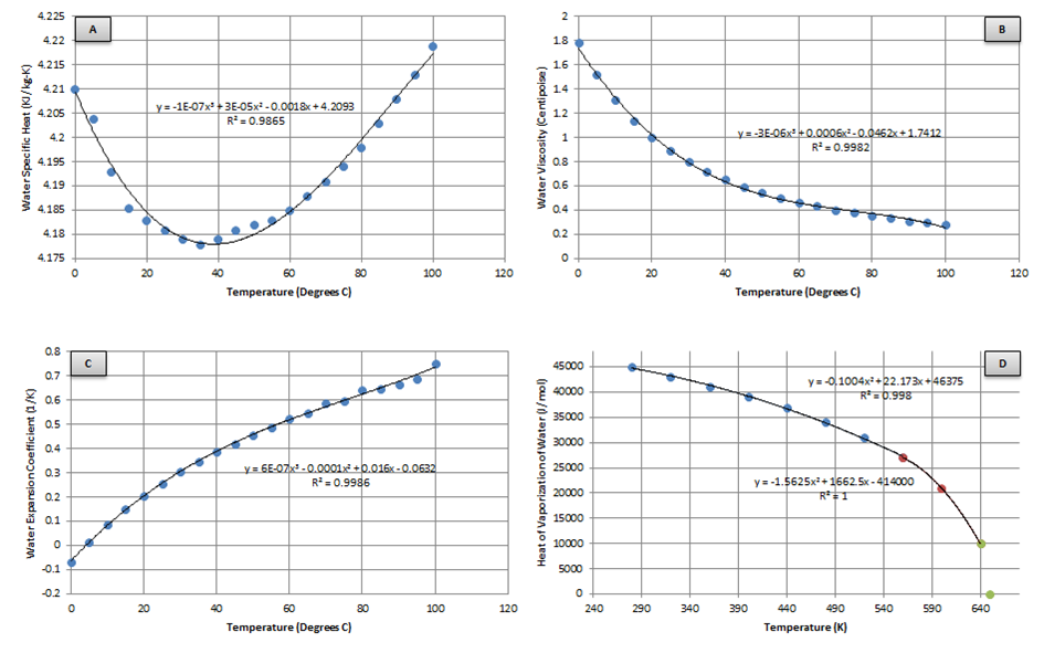
The first three properties (Figure 8 A-C) are used later for determining the heat transfer when the patient is submerged in water. Finding a best fit for these plots yields:
![\[{\mathrm{c}}_{\mathrm{p,w}}=-1e^{-7}{\mathrm{T}}^{\mathrm{3}}_{\mathrm{\infty }}+3e^{-5}{\mathrm{T}}^{\mathrm{2}}_{\mathrm{\infty }}-0.0018{\mathrm{T}}_{\mathrm{\infty }}+4.2093\]](form_63.png)
![\[\mu \mathrm{\ }=-3e^{-6}{\mathrm{T}}^{\mathrm{3}}_{\mathrm{\infty }}+0.0006{\mathrm{T}}^{\mathrm{2}}_{\mathrm{\infty }}-0.0462{\mathrm{T}}_{\mathrm{\infty }}+1.7412\]](form_64.png)
![\[\mathrm{\alpha }\mathrm{\ }=6e^{-7}{\mathrm{T}}^{\mathrm{3}}_{\mathrm{\infty }}+0.0001{\mathrm{T}}^{\mathrm{2}}_{\mathrm{\infty }}+0.016{\mathrm{T}}_{\mathrm{\infty }}-0.0632\]](form_65.png)
The heat of vaporization (Figure 8 D) is the enthalpy change required to transform a given quantity of a substance from a liquid into a gas and is needed for determining the heat lost through respiration. Finding a piecewise best fit yields:
![\[{\mathrm{h}}_{\mathrm{fg}}\mathrm{=}\left\{ \begin{array}{c}
-0.10042t^2_a+22.173t_a+46375,~t_a\mathrm{\le }\mathrm{560K} \\
-1.5625t^2_a+1662.5t_a-\mathrm{414000,}~t_a\mathrm{>560K} \end{array}
\right.\]](form_66.png)
The water vapor pressure at the skin and in ambient air is determined using the piecewise Antoine Equation given by Equation 17 [14] . The resulting pressure is in units of mmHg and is a function of temperature in degrees Celsius. The constants are given by Table 5.
![\[p\mathrm{=}{\mathrm{10}}^{\left(A\mathrm{-}\frac{B}{C\mathrm{+}t}\right)}\]](form_67.png)
| A | B | C | t min (degrees C) | t max (degrees C) |
|---|---|---|---|---|
| 8.07131 | 1730.63 | 233.426 | 1 | 100 |
| 8.14019 | 1810.94 | 44.485 | 99 | 374 |
The density of air is then determined using Equations 18-20 [319] .
![\[p_d\mathrm{=}p_t\mathrm{-}p_v\]](form_68.png)
![\[p_v\mathrm{=}\mathrm{\phi }p_a\]](form_69.png)
![\[\rho \mathrm{=}\frac{p_dM_d\mathrm{+}p_vM_v}{Ut_a}\]](form_70.png)
The Lewis Relationship is the ratio of mass transfer coefficient to heat transfer coefficient, which is needed later in the determination of the heat loss due to evaporation. For the air-water system with low concentration of water vapor, it is assumed the adiabatic saturation temperature and wet-bulb temperature are equal [164] , and is therefore given by:
![\[\beta \mathrm{=}\frac{\mathrm{1}}{\rho c_p}\]](form_71.png)
Radiation
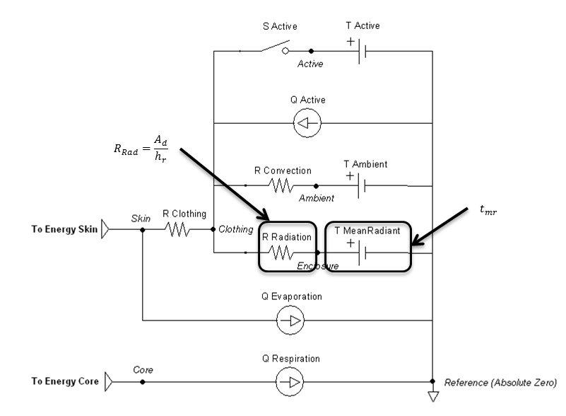
The radiation heat transfer coefficient is used to determine the radiation resistance element value in the Environment thermal circuit. Equation 22 is implemented to determine this coefficient each time step. The mean radiant temperature is a known value set by the user, and the clothing temperature is solved directly by the circuit and used as a feedback mechanism. The ratio of the effective area to the surface area (Ar/Ad) is set constant to 0.73, which is typical for a standing person. In contrast, 0.70 is typical for a sitting person [153] .
![\[{\mathrm{h}}_r\mathrm{=4}\varepsilon \sigma \frac{A_r}{A_D}{\left(\frac{t_{cl}\mathrm{+}t_{mr}}{\mathrm{2}}\right)}^{\mathrm{3}}\]](form_72.png)
Figure 9 highlights which elements are modified by the radiation method and by which parameters.
Convection
The equation chosen to account for convective effects comes from a study that used experimental data from a segmented manikin in a climate chamber [76] . A general-purpose forced convection equation was produced that is suitable for application to both seated and standing postures. The air velocity is a known value set by the user, taking into account the combination of wind and patient movement. The convective heat transfer coefficient is given by:
![\[{\mathrm{h}}_c\mathrm{=10.3}v^{\mathrm{0.6}}\]](form_73.png)
Figure 6 highlights which elements are modified by the convection method and by which parameters.
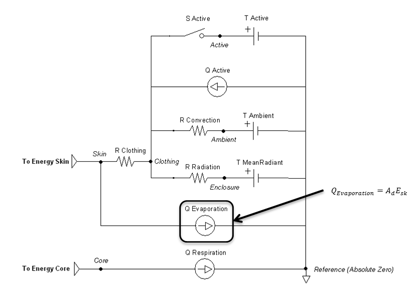
Evaporation
Evaporative heat loss is directly solved and implemented in the circuit as a heat sink on the skin. It depends on the amount of moisture on the skin and the difference between the water vapor pressure at the skin and the ambient environment. The evaporative heat transfer coefficient for the outer air layer of a nude or clothed person can be estimated from the convective heat transfer coefficient using the Lewis Relationship (Equation 24) [153].
![\[{\mathrm{h}}_e\mathrm{=}\beta {\mathrm{h}}_c\]](form_74.png)
Clothing can then be taken into account to determine the maximum evaporative potential [181] :
![\[F_{pcl}\mathrm{=}\frac{\mathrm{1}}{\mathrm{1+2.}\mathrm{22}{\mathrm{h}}_cR_{cl}}\]](form_75.png)
![\[E_{max}\mathrm{=}{\mathrm{h}}_eF_{pcl}\left(p_{sk,s}\mathrm{-}p_a\right)\]](form_76.png)
Skin wettedness is an important factor to determine evaporative heat loss [153] :
![\[w_{rsw}\mathrm{=}\frac{E_{rsw}}{E_{max}}\]](form_77.png)
![\[E_{dif}\mathrm{=}\left(\mathrm{1-}w_{rsw}\right)\mathrm{0.06}E_{max}\]](form_78.png)
Evaporative heat loss by sweating is directly proportional to the rate of sweat generation through Equation 29 [153] . The sweat rate is set by the Energy system.
![\[E_{rsw}\mathrm{=}{\dot{m}}_{rsw}{\mathrm{h}}_{fg}\]](form_79.png)
![\[E_{sk}\mathrm{=}E_{rsw}\mathrm{+}E_{dif}\]](form_80.png)
Figure 11 highlights which elements are modified by the evaporation method and by which parameters.
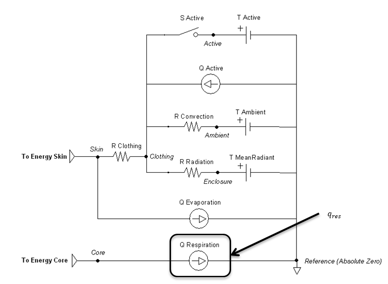
Respiration
Respiratory heat exchange is taken into account with varying temperatures and humidity of inspired air.
Note that this calculation will be the same for both surrounding fluids—air and water. It is assumed that the patient’s head remains above water when breathing. If the patient holds their breath to fully submerge, the respiration rate should be zero, which will correctly eliminate any heat transfer through the lungs.
The unitless specific humidity (mass/mass) is needed to determine the inspiratory-expiratory humidity difference. Equation 31 solves for this knowing the ambient temperature (in Kelvin), relative humidity, and local atmospheric pressure [74]—all user defined values.
![\[\mathrm{H=}\frac{\mathrm{100}\mathrm{\phi }}{\mathrm{0.263}p_t}e^{\left(\frac{\mathrm{17.67}\left(t_a\mathrm{-}\mathrm{273.16}\right)}{t_a\mathrm{-}\mathrm{29.65}}\right)}\]](form_81.png)
The humidity difference is then given by (ta in degrees F) [224] :
![\[\mathrm{\Delta }W\mathrm{=0.02645+0.0000361}t_a\mathrm{-}\mathrm{0.798}H\]](form_82.png)
Since heat and water vapor are transferred in the lungs, expired air is saturated with water vapor at the temperature of the respiratory tract [321] . The respiration rate is given by the Respiratory system and used to determine the following heat loss:
![\[q_{res,lat}\mathrm{=}{\mathrm{h}}_{fg}{\dot{m}}_{res}\mathrm{\Delta }W\]](form_83.png)
![\[q_{res,sen}\mathrm{=}{\dot{m}}_{res}\rho c_p\left(t_{res}\mathrm{-}t_{a,res}\right)\]](form_84.png)
![\[q_{res}\mathrm{=}q_{res,lat}\mathrm{+}q_{res,sen}\]](form_85.png)
Figure 12 highlights the source element that is modified by the respiration method.
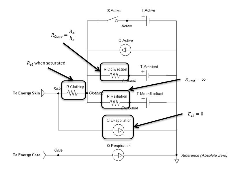
Submerged
Submerging the patient is done by using the environment change action or condition to set the surrounding type enumeration to water. The ambient temperature will be the water temperature. The clothing resistance will be the value when submerged, likely fully saturated or modified to a wet suit value. The currently implemented model assumes fresh water only, with a water pressure of 0.1 MPa (sea level). It also assumes that radiation and evaporation effects are negligible.
The thermal conductivity of the water can be solved using [283] :
![\[T\mathrm{=}\frac{T_{\mathrm{\infty }}}{\mathrm{298.15}}\]](form_86.png)
![\[k\mathrm{=0.6065}\left(\mathrm{-}\mathrm{1.48445}~\mathrm{+4.12292}~T\mathrm{+-1.63866}~T^{\mathrm{2}}\right)\]](form_87.png)
![\[\nu \mathrm{=}\frac{\mu }{\rho }\]](form_88.png)
Equation 39 solves for the Prandtl number, which is the dimensionless ratio of momentum diffusivity (kinematic viscosity) to thermal diffusivity.
![\[Pr\mathrm{=}\frac{c_{p,w}\mu }{k}\]](form_89.png)
Equation 40 solves for the Grashof number, which is the dimensionless value that approximates the ratio of the buoyancy to viscous force acting on a fluid.
![\[Gr\mathrm{=}\frac{g\mathrm{\alpha }\left(T_s\mathrm{-}T_{\mathrm{\infty }}\right)D^{\mathrm{3}}}{{\mathrm{\nu }}^{\mathrm{2}}}\]](form_90.png)
The heat transfer coefficient can is determined by [42] :
![\[{\mathrm{h}}_c\mathrm{=0.09}\left(Gr\mathrm{-}Pr\right)\mathrm{0.275}\]](form_91.png)
Figure 13 highlights which elements are modified when submerged and by which parameters. Radiation is handled much like an open switch in a circuit via the resistor and does not allow any transfer. The evaporation transfer source is directly set to zero.
Outputs
The temperature at each node and heat flow on each path in the Environment thermal circuit is calculated every time step. The following system data is also set:
- Convective Heat Loss (Power)
- Convective Heat Transfer Coefficient (Heat Conductance per Area)
- Evaporative Heat Loss (Power)
- Evaporative Heat Transfer Coefficient (Heat Conductance per Area)
- Radiative Heat Loss (Power)
- Radiative Heat Transfer Coefficient (Heat Conductance per Area)
- Respiration Heat Loss (Power)
- Skin Heat Loss (Power)
Assumptions and Limitations
The Ambient node operates under some pretenses for its interaction with other systems. Since the atmospheric pressure is used to set the pulmonary reference nodes, everything in those systems is referenced to zero pressure. This is in contrast to reporting the difference from atmospheric pressure, as is often the standard. It is further assumed that all ambient substance volume fractions set the sum to 1. The included scenarios generally use nitrogen in place of other inert gases.
Beyond the inferences mentioned previously in this document, some high-level assumptions for the Environment system as a whole:
- Whole body average heat transfer, i.e., lumped parameters
- Standing patient position
- Standard air composition for heat transfer calculations
- Air is an ideal gas for heat transfer calculations
- Ignore movement of water when submerged
- No transitional heat transfer mechanics after submersion has ended (not accounting for water mass remaining on skin)
- No endogenous production of carbon monoxide
- Endogenous production is very small so that even at very low environmental concentrations alveolar diffusion dominates
- The only carbon monoxide exposure pathophysiology simulated is tissue hypoxia
- We do not model CO mediated damage at the cellular level (i.e. no oxidative stress or lipid peroxygenation)
Conditions
The environment change condition has the option to be done directly or by reading an environment xml file. Like other conditions, the engine will stabilize the patient within that environment before running a simulation. This is modeled most like a rapid decompression, and not necessarily the same as a patient that has lived in a "non-standard" environment and undergone physiologic changes (e.g., Himalayan Sherpas with high altitude adaptations).
Actions
The environment change action has the option to be done directly or by reading an environment xml file. Any of the parameters shown in Table 1 can be modified in this manor during runtime.
The thermal application action can directly add heat, remove heat, or set a temperature over any percentage of the patient’s body. They can be called individually or will sum together if called in combination. These actions will set the active heat flow source and/or the active temperature source shown in Figure 14. The applied area or fraction is used to determine the average amount to apply to the patient, since the Environment is modeled as a one-dimensional circuit. When actively heating or cooling, the total power is directly scaled using the fraction of the body that is covered using the patient skin surface area. When applying a specific temperature, the average temperature will be applied between it and the ambient value, weighted by the fraction of the body covered.
Events
There are currently no events in the Environment system.
Results and Conclusions
Verification
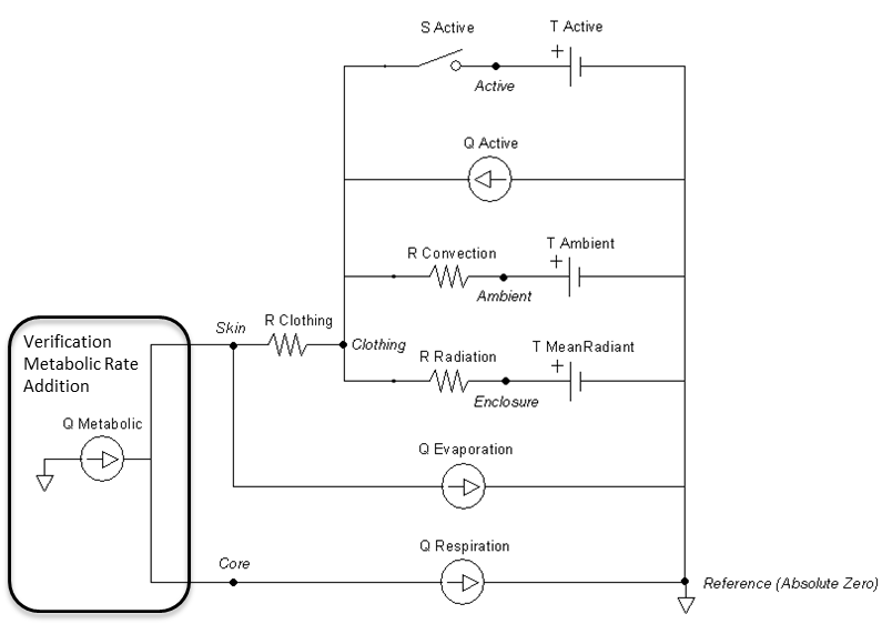
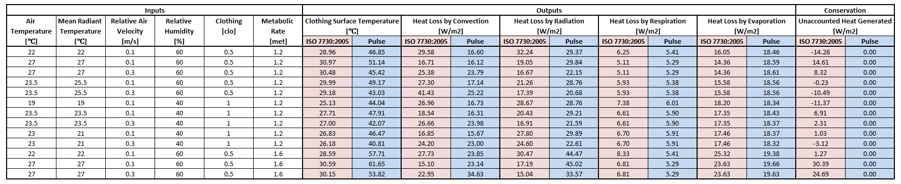
Results using the equations from ISO 7730:2005 were used to compare to Environment outputs. The standard focuses mostly on two thermal comfort metrics, Predictive Mean Vote and Predictive Percentage Dissatisfied [171]. Although it is intended for the ergonomics of thermal environments, intermediate values can be extracted for the values shown in Table 6. The connection points that connect to the Energy system are replaced with a heat source equal to the metabolic rate, shown in Figure 15. The other circuit elements are set to match the Inputs columns in Table 6. The static circuit is run until everything balances and steady state is reached. The clothing surface temperature is collected directly from the clothing node and system heat loss values are collected directly from the flow in the appropriate paths.
The following assumptions are made for this verification test:
- Complete conservation of thermal energy with none stored
- Constant respiration rate of 16 breaths/min
- Constant sweat rate of 1e-5 kg/s
The results in Table 6 show the skin temperatures calculated significantly higher than that by the ISO standard code. However, the individual heat loss values seem reasonable and show the correct trends based on the inputs. The Environment model conserves energy as seen in the last column with the difference in heat produced by the metabolic rate to the sum of the heat loss by all four means. The ISO standard does not conserve energy in the same way, and makes several looser assumptions that the Environment system does not. This could explain many of the discrepancies. The requirement for the Environment system to be able to handle extreme environments with feedback from other systems requires it to more strictly adhere to a rigorous physics based modeling approach.
Validation
Forest Fire Fighter
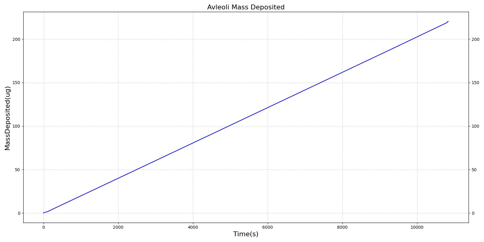
This scenario simulates exposure to a moderate/severe forest fire . This includes a suspension of wood particulate concentration of 2.9 mg/m^3 and a concentration of carbon monoxide of 20 ppm. Environmental composition data for this scenario simulation was taken from [285]. Spirometry data was determined through expiratory flow curve taken during conscious respiration. Figure 16 details the difference in mass deposited in two separate respiratory compartments (following from equations 1-7) and the difference in expiratory flow before and after smoke inhalation. Slight decreases to the expiratory flow maximum are seen and coincide fairly well with validated data [33].
 | 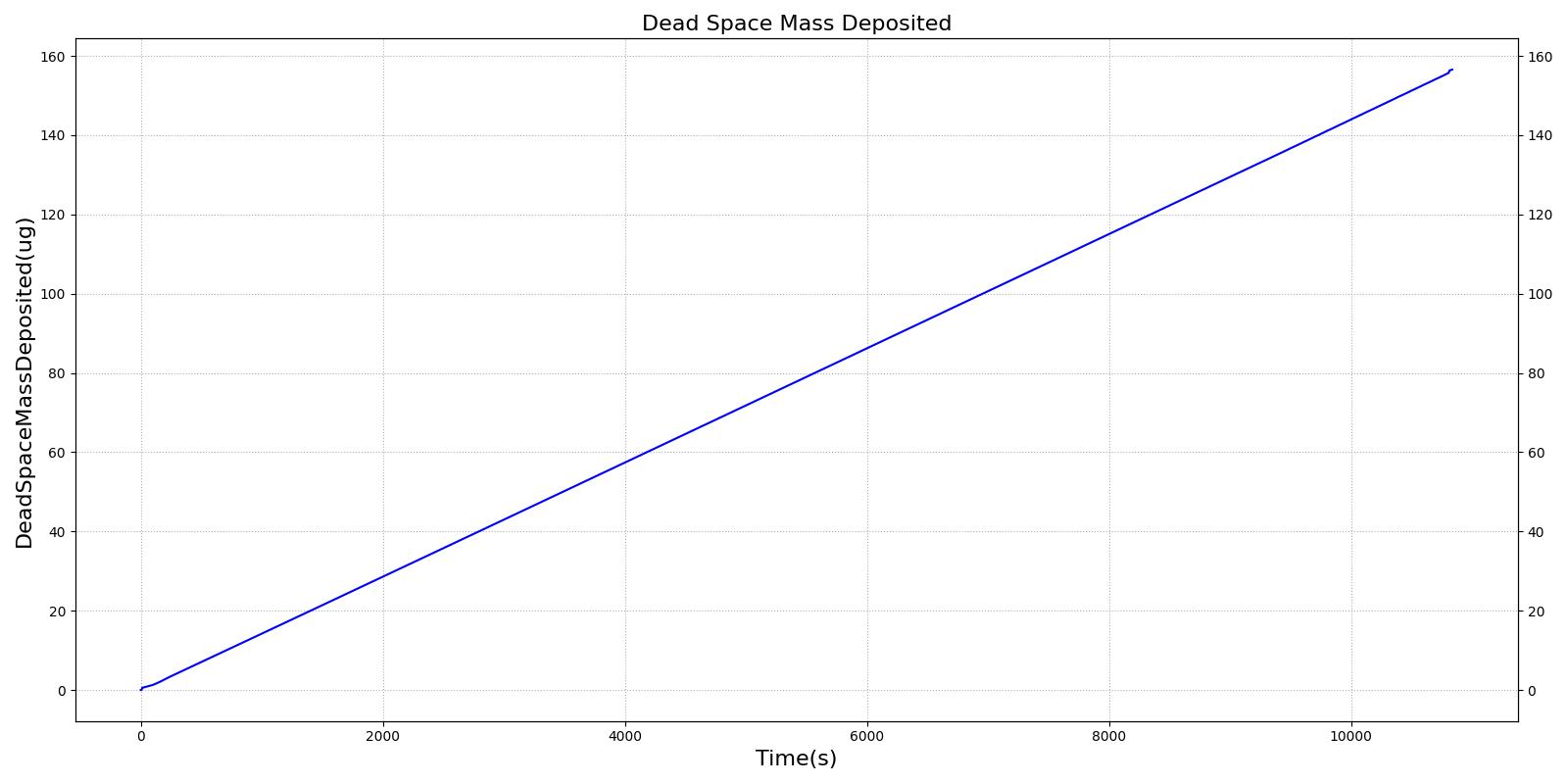 |
 | 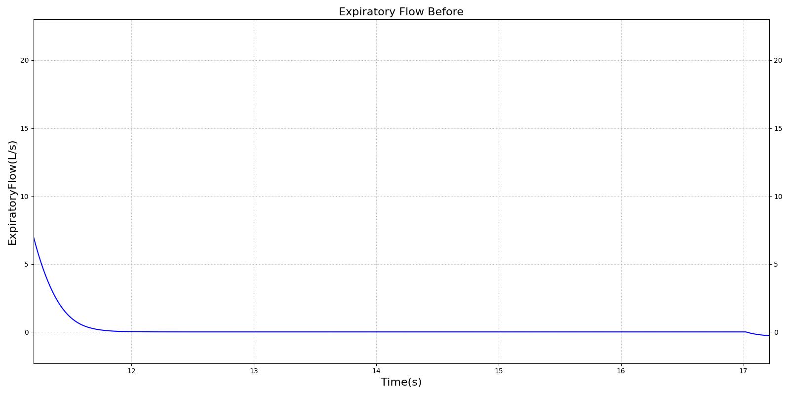 |
| Action | Notes | Occurrence Time (s) | Sampled Scenario Time (s) | Functional Vital Capacity (% from baseline PFT) | Functional expiratory volume over 1 second (Change) | Forced expiratory flow (25-75) (Change) |
|---|---|---|---|---|---|---|
| Environment Change: Exposed to moderate/severe forest fire | Patient is exposed to smoke and CO inhalation | 10 | 240 | no change | no change | No Change |
| PFT administered before and after exposure to forest fire | Validation is computed against pre-exposed patient data | 5 and 310 | 310 | Decrease by 1% [33] | Decrease 3% [33] | Decrease 6% [33] |
Carbon Monoxide
There are two scenarios used to validate carbon monoxide poisoning. The first is an exposure to CO at 200 ppm, which is the National Institute for Occupational Safety and Health ceiling osha_co. The second is an exposure to CO at 5000 ppm, which is an extreme exposure that should result in death. Because the many of the symptoms of CO poisoning are not modeled (e.g. head ache, nausea, syncope), validation is conducted by comparing the carboxyhemoglobin kinetics to the Coburn-Forster-Kane equation coburn1965considerations and to data presented in stewart1975effect.
| Action | Notes | Occurrence Time (s) | Sampled Scenario Time (s) | Pulse Oximetry | Oxygen Saturation | Percent Carboxyhemoglobin |
|---|---|---|---|---|---|---|
| Environment Change: Carbon Monoxide 200ppm | Person is exposed to 200ppm carbon monoxide. The maximal steady-state concentration | 5 | N/A | 95 to 98% [148] | 95 to 98% [148] | Approx. 0 [40] pg. 690 |
| None | 10 minutes | N/A | 605 | Normal [298] | Decreased | 1 to 2 % [335] |
| None | 30 minutes | N/A | 1805 | Normal [298] | Decreased | 3 to 4 % [335] |
| None | 1 hour | N/A | 3605 | Normal [298] | Decreased | 5 to 6 % [335] |
| None | 4 hours | N/A | 12005 | Normal [298] | Decreased | 12 to 16% [335] |
| Action | Notes | Occurrence Time (s) | Sampled Scenario Time (s) | Pulse Oximetry | Oxygen Saturation | Percent Carboxyhemoglobin |
|---|---|---|---|---|---|---|
| Environment Change: Carbon Monoxide 5000ppm | Person is exposed to 5000ppm carbon monoxide. The maximal steady-state concentration | 5 | N/A | 95 to 98% [148] | 95 to 98% [148] | Approx. 0 [40] pg. 690 |
| None | 1 hour | N/A | 3605 | Normal [298] | Decreased | approx. 80% [335] Increased [350] |
| None | 2 hours - Irreversible state should happen by this point | N/A | 7205 | Normal [298] | Death (Irreversible State) | Death (Irreversible State) |
See the Energy Methodology for validation in varying and extreme environments.
See the Drugs Methodology for validation of airborne agents.
Conclusions
The Environment System successfully allows the user to manipulate parameters external to the patient.
Future Work
Coming Soon
There are no planned near term additions.
Recommended Improvements
Here are some recommended improvements:
- Add the ability to define submerged surrounding liquid properties (e.g., sea water at depth)
- Add a segmented model, instead of an averaged whole body approach
- Account for patient posture
- Add Thermal Comfort Assessment - Predictive Mean Vote (PMV) and Predictive Percentage Dissatisfied (PPD)
- Integrate 3D models for indoor, outdoor, urban, etc. to modify values—especially mean radiant temperature and velocity (wind & motion)
- Add the ability to auto-populate environment parameters based on location and time of year
- From lat/lon and date meteorological inputs
- From real-time data
- Add radiation analysis
Appendices
Acronyms
CDM - Common Data Model
PMV - Predictive Mean Vote
PPD - Predictive Percentage Dissatisfied
The variables presented in Table 10 are used throughout this document.

Data Model Implementation
Compartments
- Active
- Ambient
- Clothing
- Enclosure
- ExternalCore
- ExternalSkin
- ExternalGround